Models
This section contains numerical models that can be used directly to run finite element simulations which can be compartmentalized or homogeneous.
CuboidTest
-
class
compmod.models.CuboidTest(**kwargs)[source]¶ Performs a uniaxial tensile or compressive test on an cuboid rectangular cuboid along the y axis. The cuboid can be 2D or 3D. Lateral conditions can be specified as free or pseudo homogeneous.
Parameters: - lx (float) – length of the box along the x axis (default = 1.)
- ly (float) – length of the box along the y axis (default = 1.)
- lz (float) – length of the box along the z axis (default = 1.). Only used in 3D simulations.
- Nx (int) – number of elements along the x direction.
- Ny (int) – number of elements along the y direction.
- Nz (int) – number of elements along the z direction.
- disp (float) – imposed displacement along the y direction (default = .25)
- export_fields – indicates if the field outputs are exported (default = True). Can be set to False to speed up post processing.
- lateral_bc (dict) – indicates the type of lateral boundary conditions to be used.
- abqlauncher (string) – path to the abaqus executable.
- material – material instance from abapy.materials
- label (string) – label of the simulation (default: ‘simulation’)
- workdir (string) – path to the simulation work directory (default: ‘’)
- compart (integer) – indicated if the simulation homogeneous or compartimented (default: False)
- nFrames (integer) – number or frames per step (default: 100)
- elType (string) – element type (default: ‘CPS4’)
- is_3D (boolean) – indicates if the model is 2D or 3D (default: False)
- cpus – number of CPUs to use (default: 1)
- force (boolean) – test in force
- displacement (boolean) – test in dispalcement
This model can be used for a wide range of problems. A few examples are given here:
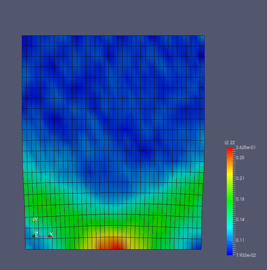
- Simple 2D compartmentalized model:
from abapy import materials
from abapy.misc import load
import matplotlib.pyplot as plt
from matplotlib import cm
import numpy as np
import pickle, copy, platform, compmod


# GENERAL SETTINGS
settings = {}
settings['export_fields'] = True
settings['compart'] = True
settings['is_3D']   = False
settings['lx']      = 10.
settings['ly']      = 10. # test direction
settings['lz']      = 10.
settings['Nx']      = 40
settings['Ny']      = 20
settings['Nz']      = 2
settings['disp']    = 1.2
settings['nFrames'] = 50
settings['workdir'] = "workdir/"
settings['label']   = "cuboidTest"
settings['elType']  = "CPS4"
settings['cpus']    = 1

run_simulation = False # True to run it, False to just use existing results

E           = 1.
sy_mean     = .001
nu          = 0.3
sigma_sat   = .005
n           = 0.05


# ABAQUS PATH SETTINGS
node = platform.node()
if node ==  'lcharleux':
  settings['abqlauncher']   = "/opt/Abaqus/6.9/Commands/abaqus"
if node ==  'serv2-ms-symme':
  settings['abqlauncher']   = "/opt/abaqus/Commands/abaqus"
if node ==  'epua-pd47':
  settings['abqlauncher']   = "C:/SIMULIA/Abaqus/6.11-2/exec/abq6112.exe"
if node ==  'epua-pd45':
  settings['abqlauncher']   = "C:\SIMULIA/Abaqus/Commands/abaqus"
if node ==  'SERV3-MS-SYMME':
  settings['abqlauncher']   = "C:/Program Files (x86)/SIMULIA/Abaqus/6.11-2/exec/abq6112.exe"


# MATERIALS CREATION
Ne = settings['Nx'] * settings['Ny']
if settings['is_3D']: Ne *= settings['Nz']
if settings['compart']:
  E         = E         * np.ones(Ne) # Young's modulus
  nu        = nu        * np.ones(Ne) # Poisson's ratio
  sy_mean   = sy_mean   * np.ones(Ne)
  sigma_sat = sigma_sat * np.ones(Ne)
  n         = n         * np.ones(Ne)
  sy = compmod.distributions.Rayleigh(sy_mean).rvs(Ne)
  labels = ['mat_{0}'.format(i+1) for i in xrange(len(sy_mean))]
  settings['material'] = [materials.Bilinear(labels = labels[i],
                                 E = E[i], nu = nu[i], Ssat = sigma_sat[i],
                                 n=n[i], sy = sy[i]) for i in xrange(Ne)]
else:
  labels = 'SAMPLE_MAT'
  settings['material'] = materials.Bilinear(labels = labels,
                                E = E, nu = nu, sy = sy_mean, Ssat = sigma_sat,
                                n = n)


m = compmod.models.CuboidTest(**settings)
if run_simulation:
  m.MakeInp()
  m.Run()
  m.MakePostProc()
  m.RunPostProc()
m.LoadResults()
# Plotting results
if m.outputs['completed']:


  # History Outputs
  disp =  np.array(m.outputs['history']['disp'].values()[0].data[0])
  force =  np.array(np.array(m.outputs['history']['force'].values()).sum().data[0])
  volume = np.array(np.array(m.outputs['history']['volume'].values()).sum().data[0])
  length = settings['ly'] + disp
  surface = volume / length
  logstrain = np.log10(1. + disp / settings['ly'])
  linstrain = disp/ settings['ly']
  strain = linstrain
  stress = force / surface

  fig = plt.figure(0)
  plt.clf()
  sp1 = fig.add_subplot(2, 1, 1)
  plt.plot(disp, force, 'ro-')
  plt.xlabel('Displacement, $U$')
  plt.ylabel('Force, $F$')
  plt.grid()
  sp1 = fig.add_subplot(2, 1, 2)
  plt.plot(strain, stress, 'ro-', label = 'simulation curve', linewidth = 2.)
  plt.xlabel('Tensile Strain, $\epsilon$')
  plt.ylabel(' Tensile Stress $\sigma$')
  plt.grid()
  plt.savefig(settings['workdir'] + settings['label'] + 'history.pdf')


  # Field Outputs
  if settings["export_fields"]:
    m.mesh.dump2vtk(settings['workdir'] + settings['label'] + '.vtk')
- VTK output:
cuboidTest.vtk. - VTK file displayed with Paraview:
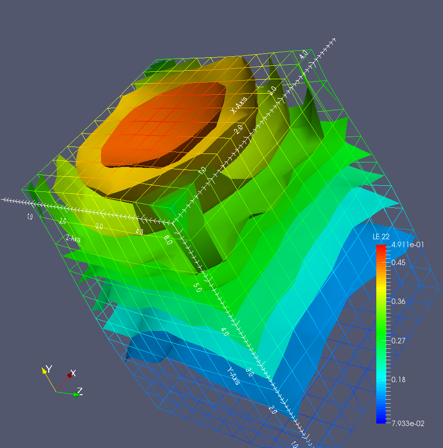
- Simple 3D compartmentalized model:
from abapy import materials
from abapy.misc import load
import matplotlib.pyplot as plt
from matplotlib import cm
import numpy as np
import pickle, copy, platform, compmod


# GENERAL SETTINGS
settings = {}
settings['export_fields'] = True
settings['compart'] = True
settings['is_3D']   = True
settings['lx']      = 5.
settings['ly']      = 5. # test direction
settings['lz']      = 5.
settings['Nx']      = 10
settings['Ny']      = 10
settings['Nz']      = 10
settings['disp']    = 1.2
settings['nFrames'] = 50
settings['workdir'] = "workdir/"
settings['label']   = "cuboidTest_3D"
settings['elType']  = "CPS4"
settings['cpus']    = 1

run_simulation = False # True to run it, False to just use existing results

E           = 1.
sy_mean     = .001
nu          = 0.3
sigma_sat   = .005
n           = 0.05


# ABAQUS PATH SETTINGS
node = platform.node()
if node ==  'lcharleux':
  settings['abqlauncher']   = "/opt/Abaqus/6.9/Commands/abaqus"
if node ==  'serv2-ms-symme':
  settings['abqlauncher']   = "/opt/abaqus/Commands/abaqus"
if node ==  'epua-pd47':
  settings['abqlauncher']   = "C:/SIMULIA/Abaqus/6.11-2/exec/abq6112.exe"
if node ==  'epua-pd45':
  settings['abqlauncher']   = "C:\SIMULIA/Abaqus/Commands/abaqus"
if node ==  'SERV3-MS-SYMME':
  settings['abqlauncher']   = "C:/Program Files (x86)/SIMULIA/Abaqus/6.11-2/exec/abq6112.exe"


# MATERIALS CREATION
Ne = settings['Nx'] * settings['Ny']
if settings['is_3D']: Ne *= settings['Nz']
if settings['compart']:
  E         = E         * np.ones(Ne) # Young's modulus
  nu        = nu        * np.ones(Ne) # Poisson's ratio
  sy_mean   = sy_mean   * np.ones(Ne)
  sigma_sat = sigma_sat * np.ones(Ne)
  n         = n         * np.ones(Ne)
  sy = compmod.distributions.Rayleigh(sy_mean).rvs(Ne)
  labels = ['mat_{0}'.format(i+1) for i in xrange(len(sy_mean))]
  settings['material'] = [materials.Bilinear(labels = labels[i],
                                 E = E[i], nu = nu[i], Ssat = sigma_sat[i],
                                 n=n[i], sy = sy[i]) for i in xrange(Ne)]
else:
  labels = 'SAMPLE_MAT'
  settings['material'] = materials.Bilinear(labels = labels,
                                E = E, nu = nu, sy = sy_mean, Ssat = sigma_sat,
                                n = n)


m = compmod.models.CuboidTest(**settings)
if run_simulation:
  m.MakeInp()
  m.Run()
  m.MakePostProc()
  m.RunPostProc()
m.LoadResults()
# Plotting results
if m.outputs['completed']:


  # History Outputs
  disp =  np.array(m.outputs['history']['disp'].values()[0].data[0])
  force =  np.array(np.array(m.outputs['history']['force'].values()).sum().data[0])
  volume = np.array(np.array(m.outputs['history']['volume'].values()).sum().data[0])
  length = settings['ly'] + disp
  surface = volume / length
  logstrain = np.log10(1. + disp / settings['ly'])
  linstrain = disp/ settings['ly']
  strain = linstrain
  stress = force / surface

  fig = plt.figure(0)
  plt.clf()
  sp1 = fig.add_subplot(2, 1, 1)
  plt.plot(disp, force, 'ro-')
  plt.xlabel('Displacement, $U$')
  plt.ylabel('Force, $F$')
  plt.grid()
  sp1 = fig.add_subplot(2, 1, 2)
  plt.plot(strain, stress, 'ro-', label = 'simulation curve', linewidth = 2.)
  plt.xlabel('Tensile Strain, $\epsilon$')
  plt.ylabel(' Tensile Stress $\sigma$')
  plt.grid()
  plt.savefig(settings['workdir'] + settings['label'] + 'history.pdf')


  # Field Outputs
  if settings["export_fields"]:
    m.mesh.dump2vtk(settings['workdir'] + settings['label'] + '.vtk')
- VTK output:
cuboidTest.vtk. - VTK file displayed with Paraview:
- CuboidTest with microstructure generated using Voronoi cells :
- Source:
cuboidTest_voronoi. - VTK output:
cuboidTest_voronoi.
-
DeleteOldFiles()¶ Deletes old job files.
-
PostProc()¶ Makes the post proc script and runs it.
-
Run(deleteOldFiles=True)¶ Runs the simulation.
Parameters: deleteOldFiles – indicates if existing simulation files are deleted before the simulation starts.
-
RunPostProc()¶ Runs the post processing script.
RingCompression
-
class
compmod.models.RingCompression(**kwargs)[source]¶ let see 2 kind of RingCompression , one homogenous and the second compartmentalized
RingCompression_3D
from compmod.models import RingCompression
from abapy.materials import Hollomon
from abapy.misc import load
import matplotlib.pyplot as plt
import numpy as np
import pickle, copy
import platform

#PAREMETERS
is_3D = True
inner_radius, outer_radius = 45.2 , 48.26
Nt, Nr, Na = 20, 3, 6
displacement = 45.
nFrames = 100
sy = 150.
E = 64000.
nu = .3
n = 0.1015820312
thickness =14.92
workdir = "workdir/"
label = "ringCompression_3D"
elType = "C3D8"
filename = 'test_expD2.txt'
cpus = 1
node = platform.node()
if node ==  'lcharleux':      abqlauncher   = '/opt/Abaqus/6.9/Commands/abaqus' # Ludovic
if node ==  'serv2-ms-symme': abqlauncher   = '/opt/abaqus/Commands/abaqus' # Linux
if node ==  'epua-pd47':
  abqlauncher   = 'C:/SIMULIA/Abaqus/6.11-2/exec/abq6112.exe' # Local machine configuration
if node ==  'SERV3-MS-SYMME':
  abqlauncher   = '"C:/Program Files (x86)/SIMULIA/Abaqus/6.11-2/exec/abq6112.exe"' # Local machine configuration
if node ==  'epua-pd45':
  abqlauncher   = 'C:\SIMULIA/Abaqus/Commands/abaqus'

#TASKS
run_sim = True
plot = True

def read_file(file_name):
  '''
  Read a two rows data file and converts it to numbers
  '''
  f = open(file_name, 'r') # Opening the file
  lignes = f.readlines() # Reads all lines one by one and stores them in a list
  f.close() # Closing the file
#    lignes.pop(0) # Delete le saut de ligne for each lines
  force_exp, disp_exp = [],[]

  for ligne in lignes:
      data = ligne.split() # Lines are splitted
      disp_exp.append(float(data[0]))
      force_exp.append(float(data[1]))
  return -np.array(disp_exp), -np.array(force_exp)


disp_exp, force_exp = read_file(filename)

#MODEL DEFINITION
disp = displacement/2
material = Hollomon(
  labels = "SAMPLE_MAT",
  E = E, nu = nu,
  sy = sy, n = n)
m = RingCompression( material = material ,
  inner_radius = inner_radius,
  outer_radius = outer_radius,
  disp = disp,
  thickness = thickness,
  nFrames = nFrames,
  Nr = Nr,
  Nt = Nt,
  Na = Na,
  workdir = workdir,
  label = label,
  elType = elType,
  abqlauncher = abqlauncher,
  cpus = cpus,
  is_3D = is_3D)

# SIMULATION
m.MakeMesh()
if run_sim:
  m.MakeInp()
  m.Run()
  m.PostProc()

# SOME PLOTS
mesh = m.mesh
outputs = load(workdir + label + '.pckl')

if outputs['completed']:

  # Fields
  def field_func(outputs, step):
    """
    A function that defines the scalar field you want to plot
    """
    return outputs['field']['S'][step].vonmises()
  """
  def plot_mesh(ax, mesh, outputs, step, field_func =None, zone = 'upper right', cbar = True, cbar_label = 'Z', cbar_orientation = 'horizontal', disp = True):

    A function that plots the deformed mesh with a given field on it.

    mesh2 = copy.deepcopy(mesh)
    if disp:
      U = outputs['field']['U'][step]
      mesh2.nodes.apply_displacement(U)
    X,Y,Z,tri = mesh2.dump2triplot()
    xb,yb,zb = mesh2.get_border()
    xe, ye, ze = mesh2.get_edges()
    if zone == "upper right": kx, ky = 1., 1.
    if zone == "upper left": kx, ky = -1., 1.
    if zone == "lower right": kx, ky = 1., -1.
    if zone == "lower left": kx, ky = -1., -1.
    ax.plot(kx * xb, ky * yb,'k-', linewidth = 2.)
    ax.plot(kx * xe, ky * ye,'k-', linewidth = .5)
    if field_func != None:
      field = field_func(outputs, step)
      grad = ax.tricontourf(kx * X, ky * Y, tri, field.data)
      if cbar :
        bar = plt.colorbar(grad, orientation = cbar_orientation)
        bar.set_label(cbar_label)


  fig = plt.figure("Fields")
  plt.clf()
  ax = fig.add_subplot(1, 1, 1)
  ax.set_aspect('equal')
  plt.grid()
  plot_mesh(ax, mesh, outputs, 0, field_func, cbar_label = '$\sigma_{eq}$')
  plot_mesh(ax, mesh, outputs, 0, field_func = None, cbar = False, disp = False)
  plt.xlabel('$x$')
  plt.ylabel('$y$')
  plt.savefig(workdir + label + '_fields.pdf')
  """
  # Load vs disp
  force = -2. * outputs['history']['force']
  disp = -2. * outputs['history']['disp']
  fig = plt.figure('Load vs. disp2')
  plt.clf()
  plt.plot(disp.data[0], force.data[0], 'ro-', label = 'Loading', linewidth = 2.)
  plt.plot(disp.data[1], force.data[1], 'bv-', label = 'Unloading', linewidth = 2.)
  plt.plot(disp_exp, force_exp, 'k-', label = 'Exp', linewidth = 2.)
  plt.legend(loc="upper left")
  plt.grid()
  plt.xlabel('Displacement, $U$')
  plt.ylabel('Force, $F$')
  plt.savefig(workdir + label + '_load-vs-disp.pdf')
RingCompression_3D compartimentalized
from compmod.models import RingCompression_VER
from abapy import materials
from abapy.misc import load
import matplotlib.pyplot as plt
import numpy as np
import pickle, copy
import platform

#PAREMETERS
inner_radius, outer_radius = 45.18 , 50.36
Nt, Nr, Na = 20, 4, 8
Ne = Nt * Nr * Na
disp = 10
nFrames = 100
thickness = 20.02
E  = 120000. * np.ones(Ne) # Young's modulus
nu = .3 * np.ones(Ne) # Poisson's ratio
Ssat =1000 * np.ones(Ne)
n = 200 * np.ones(Ne)
sy_mean = 200.

ray_param = sy_mean/1.253314
sy = np.random.rayleigh(ray_param, Ne)
labels = ['mat_{0}'.format(i+1) for i in xrange(len(sy))]
material = [materials.Bilinear(labels = labels[i], E = E[i], nu = nu[i], Ssat = Ssat[i], n=n[i], sy = sy[i]) for i in xrange(Ne)]

#workdir = "D:\donnees_pyth/workdir/"
#label = "ringCompression3DCompart"
#elType = "CPE4"
#cpus = 1
#node = platform.node()
#if node ==  'lcharleux':      abqlauncher   = '/opt/Abaqus/6.9/Commands/abaqus' # Ludovic
#if node ==  'serv2-ms-symme': abqlauncher   = '/opt/abaqus/Commands/abaqus' # Linux
#if node ==  'epua-pd47':
#  abqlauncher   = 'C:/SIMULIA/Abaqus/6.11-2/exec/abq6112.exe' # Local machine configuration
#if node ==  'SERV3-MS-SYMME':
#  abqlauncher   = '"C:/Program Files (x86)/SIMULIA/Abaqus/6.11-2/exec/abq6112.exe"' # Local machine configuration
#if node ==  'epua-pd45':
#  abqlauncher   = 'C:\SIMULIA/Abaqus/Commands/abaqus'

workdir = "workdir/"
label = "ringCompression_3D_compart"
elType = "CPE4"
cpus = 6
node = platform.node()
if node ==  'lcharleux':      abqlauncher   = '/opt/Abaqus/6.9/Commands/abaqus' # Ludovic
if node ==  'serv2-ms-symme': abqlauncher   = '/opt/abaqus/Commands/abaqus' # Linux
if node ==  'epua-pd47':
  abqlauncher   = 'C:/SIMULIA/Abaqus/6.11-2/exec/abq6112.exe' # Local machine configuration
if node ==  'SERV3-MS-SYMME':
  abqlauncher   = '"C:/Program Files (x86)/SIMULIA/Abaqus/6.11-2/exec/abq6112.exe"' # Local machine configuration
if node ==  'epua-pd45':
  abqlauncher   = 'C:\SIMULIA/Abaqus/Commands/abaqus'


#TASKS
run_sim = False
plot = True

#MODEL DEFINITION

m = RingCompression_VER( material = material,inner_radius = inner_radius,
  outer_radius = outer_radius,
  disp = disp/2,
  thickness = thickness,
  nFrames = nFrames,
  Nr = Nr,
  Nt = Nt,
  Na = Na,
  workdir = "workdir/",
  label = label,
  elType = elType,
  abqlauncher = abqlauncher,
  cpus = 1,
  compart = True,
  is_3D = True)

# SIMULATION
m.MakeMesh()
if run_sim:
  m.MakeInp()
  m.Run()
  m.PostProc()

# SOME PLOTS
mesh = m.mesh
outputs = load(workdir + label + '.pckl')
if outputs['completed']:

  # Fields
  def field_func(outputs, step):
    """
    A function that defines the scalar field you want to plot
    """
    return outputs['field']['S'][step].vonmises()
  """
  def plot_mesh(ax, mesh, outputs, step, field_func =None, zone = 'upper right', cbar = True, cbar_label = 'Z', cbar_orientation = 'horizontal', disp = True):

    A function that plots the deformed mesh with a given field on it.

    mesh2 = copy.deepcopy(mesh)
    if disp:
      U = outputs['field']['U'][step]
      mesh2.nodes.apply_displacement(U)
    X,Y,Z,tri = mesh2.dump2triplot()
    xb,yb,zb = mesh2.get_border()
    xe, ye, ze = mesh2.get_edges()
    if zone == "upper right": kx, ky = 1., 1.
    if zone == "upper left": kx, ky = -1., 1.
    if zone == "lower right": kx, ky = 1., -1.
    if zone == "lower left": kx, ky = -1., -1.
    ax.plot(kx * xb, ky * yb,'k-', linewidth = 2.)
    ax.plot(kx * xe, ky * ye,'k-', linewidth = .5)
    if field_func != None:
      field = field_func(outputs, step)
      grad = ax.tricontourf(kx * X, ky * Y, tri, field.data)
      if cbar :
        bar = plt.colorbar(grad, orientation = cbar_orientation)
        bar.set_label(cbar_label)


  fig = plt.figure("Fields")
  plt.clf()
  ax = fig.add_subplot(1, 1, 1)
  ax.set_aspect('equal')
  plt.grid()
  plot_mesh(ax, mesh, outputs, 0, field_func, cbar_label = '$\sigma_{eq}$')
  plot_mesh(ax, mesh, outputs, 0, field_func = None, cbar = False, disp = False)
  plt.xlabel('$x$')
  plt.ylabel('$y$')
  plt.savefig(workdir + label + '_fields.pdf')

  """
  # Load vs disp
  force = -2. * outputs['history']['force']
  disp = -2. * outputs['history']['disp']
  fig = plt.figure('Load vs. disp')
  plt.clf()
  plt.plot(disp.data[0], force.data[0], 'ro-', label = 'Loading', linewidth = 2.)
  plt.plot(disp.data[1], force.data[1], 'bv-', label = 'Unloading', linewidth = 2.)
  plt.legend(loc="upper left")
  plt.grid()
  plt.xlabel('Displacement, $U$')
  plt.ylabel('Force, $F$')
  plt.savefig(workdir + label + '_load-vs-disp.pdf')
-
DeleteOldFiles()¶ Deletes old job files.
-
LoadResults()¶ Loads the results from a pickle file.
-
PostProc()¶ Makes the post proc script and runs it.
-
Run(deleteOldFiles=True)¶ Runs the simulation.
Parameters: deleteOldFiles – indicates if existing simulation files are deleted before the simulation starts.
-
RunPostProc()¶ Runs the post processing script.
-